RodTracker

Before you start please make sure that the RodTracker is properly installed. For this refer to the installation instructions. If you were given a bundled version, i.e. an executable, you can start right away.

Starting the RodTracker

Run the RodTracker GUI using one of the possibilities:

• Run RodTracker.py manually:

  YOUR/REPO/PATH/RodTracker/src/RodTracker$ python RodTracker.py
  

• Use the registered command:

  ARBITRARY/PATH$ RodTracker
  

• Execute a stand-alone executable bundled for your system.

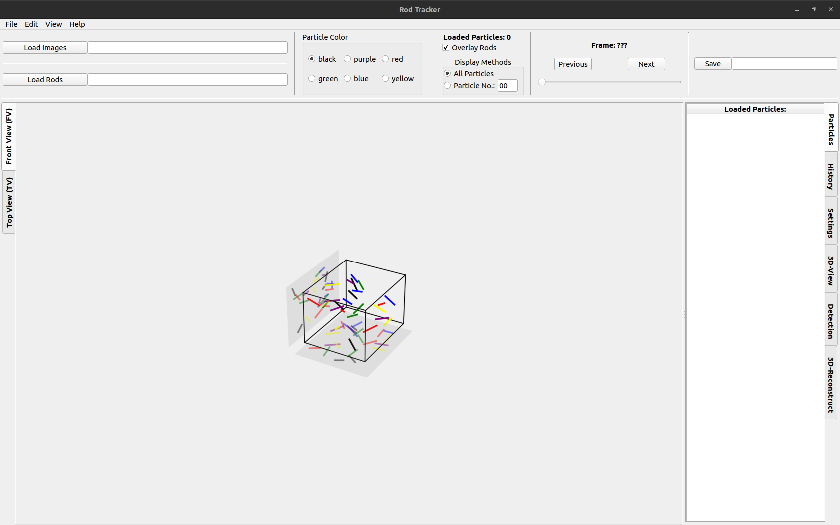
In all these cases the window shown below should be opened after the splash screen disappears. In some cases the application opens behind other windows, so look at your task bar in case you do not see this window.

Loading image data

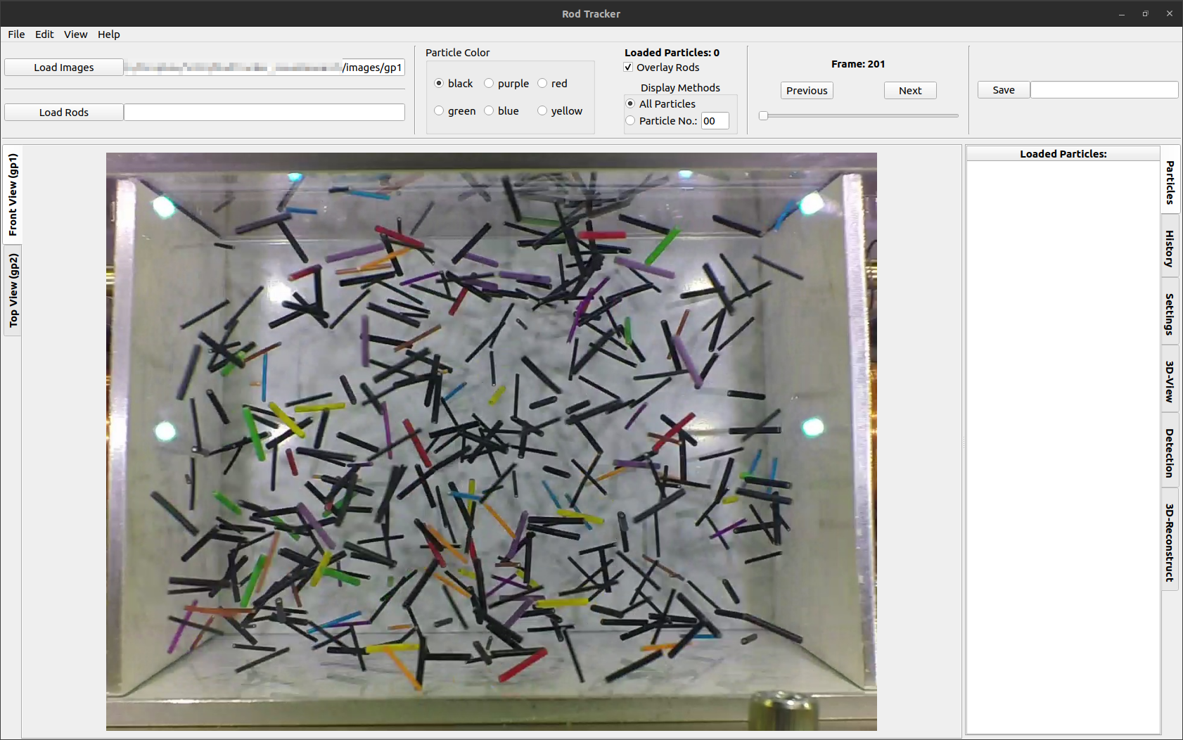
Open images from disk using the File dropdown menu, the Load Images button or the Crtl + O keyboard shortcut. Refer to Dataset format & folder structure for the correct dataset structure. You can also use the example dataset located in ./RodTracker/src/RodTracker/resources/example_data.

You can now switch between images in the folder using the left/right keys, the Previous/Next buttons or the Slider below.

Dataset format & folder structure

For the RodTracker to work properly certain folder structures, naming conventions, and file structures must be followed, which is shown below. All of these can also be viewed in the RodTracker/src/RodTracker/resources/example_data directory and that is available at resources/example_data that in the bundled RodTracker app folder.

A working folder and file structure for the stereo-camera images is shown below.

|.
├── gp1
│   ├── 001.jpg
│   ├── 002.jpg
│   ...
│   └── 321.jpg
└── gp2
    ├── 001.jpg
    ├── 002.jpg
    ...
    └── 321.jpg

When loading images the RodTracker will look for *.png, *.jpeg, and *.jpg files in the directory the file is in the user just chose. It will attempt to convert the filename to an integer, therefore keep a naming convention that allows instant conversion to integers. Leading 0s are usually not a problem for this. The folder name is then used as an ID for the loaded images and respective particle position data associated with them.

Automated detection of particles

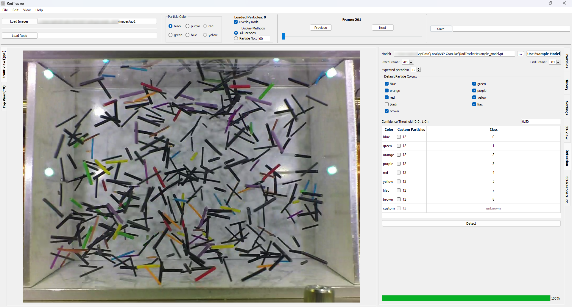
Now the particles in the loaded images can be detected using a saved model.

1. Load the model in the Detection tab and select a frame range that the model shall identify rods on.

   • The Use Example Model button downloads this model used for rod detection (specifically the model_cpu.pt file). It is intended for detecting rods in the example images.

2. Deselect any color class that you are not interested in.

3. Select the default expected number of particles, i.e. how many particles per color are expected in each image.

4. Adjust the number of particles per color, if needed, in the table and check the box to use the customized value during detection.

5. Start the detection.

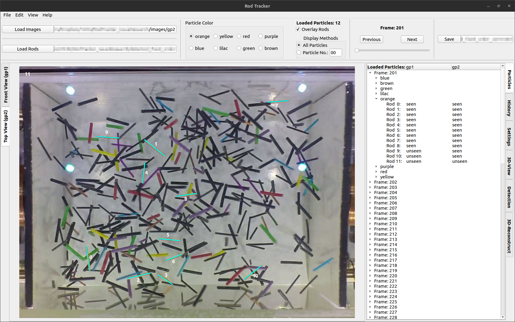
After each image is processed the data in the Particles tab is updated. Once data is available it should be displayed as an overlay immediately. If there is data available (shown in the Particles tab) but nothing is displayed, try to switch the color using the radio buttons on the top or switch frames back and forth.

Once the first data is displayed you can start with Correcting rod data, even if the detection process is still running (indicated by the green dot on the tab).

Important

Make sure the ‘first’ camera images are detected first. The first camera here referring to the camera 1 from the stereo camera calibration. The ‘first’ camera columns must be the first in the dataset given, otherwise the transformations will not work correctly (see Rod tracking and 3D coordinate reconstruction).

Correcting rod data

As the automated detection is not perfect a manual correction of the dataset is usually necessary. There are 3 possible detection and 1 tracking error classes:

1. A rod was not detected.

2. A rod was detected, but its extent is wrong, i.e. endpoint placement.

3. A rod from a different color was detected.

4. A rod is assigned a wrong number.

There are two options to select a rod for making changes to it:

• Select it by left-clicking on its number.

• Move the cursor close to it while being in the auto-selection mode activated. The mode can be toggled using the menu item in the View menu or the keyboard shortcut G.

Position correction

• left-click on the start and then end position of the misplaced rod.

• right-click anywhere to abort rod drawing.

• right click anywhere or left click on another rod to deselect the current rod.

Alternative method:

• Without previously selecting a rod left-click on the start and end position of a rod.

• Enter the desired rod number in the dialog.

  • The previous position will be replaced, if an existing rod number was entered.

  • A new rod is created, if the entered number is among in the loaded rods.

  • Only rod numbers from 0 to 99 are supported at the moment.

Number correction

• double-click on a rod number to edit it

• Press Enter, Return or left-click outside the number to confirm your input.

• Press Escape to abort editing.

Conflict handling:

The rods are marked in red when number duplicates occur after numbers were changed, i.e. when the inserted number already exists in this frame. A dialog is then displayed where you choose how to handle this conflict:

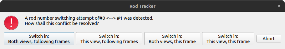
Button	Action performed
Both views, following frames	Switches the involved rod numbers in all cameras from the current frame to the last frame of the dataset.
This view, following frames	Switches the involved rod numbers in the currently displayed camera from the current frame to the last frame of the dataset.
Both views, this frame	Switches the involved rod numbers in all cameras for the current frame only.
This view, this frame	Switches the involved rod numbers only in the current camera and only the current frame.
Abort	The changed rod number is returned to its previous state. Nothing gets saved to disk.

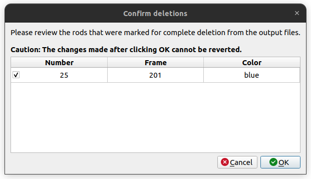
Deleting rods

A rod can be deleted by selecting it and pressing the Del key. Alternatively it can be deleted by confirming an empty rod number during the number correction.

Note

This will not actually delete the rod from the dataset yet. Instead a dummy coordinate [-1, -1] is inserted. A rod number can only be deleted completely, if it only has dummy coordinates in all frames and views it is present. This will automatically be attempted on the next saving. See the resulting dialog below:

Saving

The dataset can be saved as *.csv files. Each class(/color) is saved to an individual file as shown below. Users must manually trigger saving, but if any unsaved changes are present while attempting to close the app a dialog to resolve this will be automatically shown.

Example output structure:

|.
└── output
    ├── rods_df_black.csv
    ├── rods_df_blue.csv
    ...
    └── rods_df_yellow.csv

Example file:

	x1	y1	z1	x2	y2	z2	x	y	z	l	x1_gp1	y1_gp1	x2_gp1	y2_gp1	x1_gp2	y1_gp2	x2_gp2	y2_gp2	particle	seen_gp1	seen_gp2	frame	color
0	30.6934958642493	23.7470246454102	-1.20053394957181	38.838283423258	19.122088051726	-1.08505974899836	34.7658896437536	21.4345563485681	-1.14279684928509	9.36701324692025	949.140271493213	304.072398190045	1012.12669683258	347.511312217195	963.87465729952	432.402765085168	1049.16369886486	435.561618476477	0	1	1	100	blue
1	7.5033365995606	4.37347001474608	43.1558969732796	12.2108893096216	6.96671737173827	36.3188579087513	9.8571129545911	5.67009369324218	39.7373774410155	8.69661356750059	734.117647058824	477.828054298643	773.212669683258	451.764705882353	725.429864253394	862.262443438914	777.556561085973	799.276018099547	1	1	1	100	blue
2	32.8881625470831	25.1023926491106	0.36962926867163	40.3673686665465	18.8444760272515	-0.369807104782886	36.6277656068148	21.9734343381811	-8.89180556278291e-05	9.77991875088678	966.515837104072	291.0407239819	1027.33031674208	349.683257918552	990.808900991143	448.514929610067	1063.98119849927	442.798343867244	0	1	1	101	blue
3	6.86418195844121	-0.25337132954764	43.7173238752978	11.09727852059	-3.90663642453777	35.2044023911591	8.98073023951562	-2.08000387704271	39.4608631332285	10.1850520152751	725.429864253394	527.782805429864	775.384615384615	564.705882352941	718.810587460621	862.833132754023	754.262862459888	779.348743239618	1	1	1	101	blue

Loading rod position data

To load a position dataset in the form shown in Saving, click on the Load Rods button and select the folder with the desired *.csv files.

If no rods are shown after selecting a folder check, that the Overlay Rods box is checked, the correct image dataset is loaded (folder must match the ID appended to the 2D data column names), and that a frame is currently displayed, that has data associated with it.

Hint

You might need to adjust the Position Scaling value to 10.0 in the settings tab, if you are loading the example data.

Note

The selection dialog on Windows will not show any files in the selected directory. Therefore, make sure which directory to select in advance.

Rod tracking and 3D coordinate reconstruction

Eventually the 2D position data of the rods shall be used to reconstruct their 3D coordinates throughout the experiment. This can be achieved in the 3D-Reconstruct tab. Prerequisites for this are to have the stereo-camera calibration data (and transformation from the first camera’s coordinate system to the experiment’s coordinate system).

After successful reconstruction of 3D coordinates, the 3D-View tab will display the 3D data for the current frame and the Reconstruction performance plots are available (after updating them).

Prepare the reconstruction:

• select a frame range

• (de-)select colors

• toggle whether to track particles or just reconstruct their 3D coordinates

• select a camera calibration (see Calibration & transformation data format)

• select a transformation to experiment coordinates file (this is not strictly necessary but will benefit the visualization in the 3D-View tab) (see Calibration & transformation data format) Start the reconstruction by pressing the Solve button after making all required settings.

Note

Unlike during the detection of particles, the results will only be accessible after completion of the process or aborting. When the process is aborted all intermediate results will be integrated in the dataset and accessible in the GUI.

Calibration & transformation data format

The stereo camera calibration relates positions in images from both cameras to each other. From this the 3D coordinates of the objects shown in the images can be reconstructed. One can use OpenCV to perform the stereo camera calibration (see ParticleDetection’s camera calibration). It is also possible to do this calibration with other software, e.g. MATLAB Stereo Camera Calibrator App, as long as the pin-hole camera model is used and the calibration data is transferred into the format shown below. We have found that stereo camera calibration done via MATLAB App is generally more accurate than one done with OpenCV functions.

The transformation represents a change of coordinate system, i.e. from the first camera’s coordinate system to the world/experiment coordinate system. It must be represented as a rotation followed by a translation as shown below.

Calibration data example:

See this OpenCV documentation for more information about the individual values.

{
  "CM1": [
    [2648.548, 0.0, 656.577],
    [0.0, 2615.651, 510.264],
    [0.0, 0.0, 1.0]
  ],
  "dist1": [-0.089, 0.476, 0.0, 0.0],
  "CM2": [
    [3405.134, 0.0, 610.545],
    [0.0, 3375.154, 502.035],
    [0.0, 0.0, 1.0]
  ],
  "dist2": [-0.062, -3.676, 0.0, 0.0],
  "R": [
    [0.999, 0.004, -0.003],
    [-0.003, 0.002, -0.999],
    [-0.004, 0.999, 0.002]
  ],
  "T": [[5.960], [280.287], [353.281]],
  "E": [
    [0.137, 279.294, 354.067],
    [353.302, -4.362, -1.414],
    [-280.306, -1.250, -4.851]
  ],
  "F": [
    [1.522e-08, 3.135e-05, 0.087],
    [3.952e-05, -4.941e-07, -0.026],
    [-0.125, -0.019, 24.282]
  ]
}

Transformation data example:

{
  "rotation": [
    [0.999, 0.002, -0.006],
    [0.002, -0.999, -0.004],
    [-0.006, 0.004, -0.999]
  ],
  "translation": [
    2.059,
    2.451,
    285.952
  ]
}

Tracking vs. Reconstruction-only

The checkbox titled Tracking toggles the use of tracking and reconstruction-only mode.

In the reconstruction-only mode the particle number assignments are kept as-is. This means, that 3D coordinates are reconstructed from without attempting to find the correct/a better assignments. This is very useful, if only some manual adjustments have been made to the 2D rod data or their number assignment and their 3D coordinates need an update.

The tracking mode on the other hand attempts to find an optimal assignment of particle numbers between camera angles within one frame. Additionally, tracking particles over all frames is attempted, i.e. assigning the same ID to the same particle. For more information about the used metric, have a look at create_weights() and match_frame() in the matchND module.

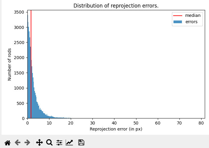
Evaluation plots

After successful reconstruction of 3D coordinates, there are evaluation plots available describing the quality of particle tracking and reconstruction. There are examples shown below for the three kinds of graphs currently produced.

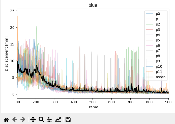
Rod lengths

A histogram of rod lengths of all selected colors in the currently loaded dataset.

Reprojection errors

A histogram of reprojection errors per rod of all selected colors in the currently loaded dataset.

Displacement per frame

Displacement of the center of each rod and the average per color per frame. One figure is produced for each selected color.

3D display

After successful reconstruction the 3D data can be displayed in the 3D. If an appropriate transformation to experiment coordinates was given, the detected particles will show up inside the indicated experimental container (see example image below).

This view is specifically useful for evaluating which rod might have not been matched correctly between the two camera angles. It can be easily identified by selecting the Top or Front view in 3D to match the displayed camera images.

Additionally, it is useful to evaluate the tracking of rods over multiple frames. In most cases where there is a problem with the tracking the resulting 3D rods will significantly jump in between two frames which is easy to pick up visually when scrolling through the frames.

There is also settings to adjust the experiment volume to match the data.

Note

The display of 3D rods can also be switched off using the Show 3D checkbox in the 3D-View tab, in case the display impairs performance of the application.

Keyboard shortcuts

Feature	Shortcut
Open images	Ctrl + O
Save rod position data	Ctrl + S
Switch to next/previous view	Ctrl+Tab
Zoom in/out	+/- Ctrl+Wheel
Fit image to available space	F
Show in original size	Ctrl + R
Next/previous image	Right/Left
Undo	Ctrl + Z
Lengthen/Shorten a rod	A/S
Lengthen/Shorten all rods in current view	R/T
Delete a selected rod	Del
Toggle automatic rod selection mode	G

Problem handling

If a problem occurs with the RodTracker, e.g. it crashes, please first have a look at the log file. The log file is saved in your platform’s directory for temporary files in the folder ./RodTracker/. It can also be accessed from the RodTracker Help dropdown menu.

To avoid excessive loss of data, the RodTracker automatically saves your currently loaded data to the temporary folder mentioned above. The most recent data is then available under ./RodTracker/autosaved/.

Known issues

• make sure the front camera images are detected first

  • the front camera columns must be the first in the dataset given

  • otherwise the transformations will not work correctly

• infinite “busy” indicator of 3D-reconstruction during/after detection

  • it’s not “busy”, but the indicator is never removed because no graphs are generated

• PulpSolverError when attempting to run a 3D reconstruction in the same session as the detection

• typing during interacting with a dialog can/will freeze the GUI

  • might be due to the EventFilter(s) that handles some keyboard shortcuts

• memory leak from plotting

  • see this issue of matplotlib

  • this problem is partially mitigated by deactivating automatic plot updating after new data has been loaded

For more (recent) information about issues see the GitHub repository.